Uncertainty Quantification in Climate Neural Networks with Bayesian Layers and MC Dropout

Neural networks are increasingly used in climate science workflows, from statistical downscaling and bias correction to emulating expensive Earth System Models (ESMs). They can be fast and accurate, but climate decisions rarely hinge on a single point prediction.

In climate work, what matters is risk under uncertainty. A forecasted temperature anomaly of $+2.1^\circ C$ is not equally useful everywhere; what you really need is $+2.1^\circ C \pm \text{(something)}$, plus an honest explanation of whether uncertainty comes from natural variability, measurement noise, or model ignorance.

Uncertainty quantification (UQ) turns a neural network from a “prediction machine” into a decision-support tool. It helps coastal planners decide how conservative to be, helps public health teams decide how early to warn for heat waves, and helps climate analysts know where additional data or better modeling is most valuable.

This article is for intermediate-to-advanced learners and career-switchers who already know the basics of deep learning and want serious, practical depth. We’ll implement probabilistic climate regression in PyTorch, estimate epistemic uncertainty with Monte Carlo (MC) dropout, and add a simple Bayesian layer to make uncertainty more explicit.

By the end, you will know how to distinguish epistemic vs aleatoric uncertainty, build a heteroscedastic regression network that predicts both mean and variance, run MC dropout inference to approximate Bayesian model averaging, and evaluate uncertainty using coverage and likelihood-based metrics rather than relying only on RMSE.

Background and prerequisites

Prerequisites you should have

You should be comfortable with Python and basic PyTorch training loops. If you can define an nn.Module, train it with an optimizer, and use DataLoader, you have enough PyTorch skill to follow the implementation sections.

You should also have a basic probability foundation. You don’t need deep Bayesian theory, but you should understand what a Gaussian distribution is, what variance means, and why log-likelihood is a natural objective when predicting distributions.

Finally, you should be aware that climate datasets are not i.i.d. tabular datasets. They are spatiotemporal fields with strong autocorrelation, seasonal structure, and non-stationarity, which affect how we split data and interpret uncertainty.

Climate domain concepts that affect modeling

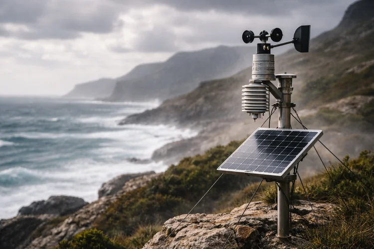
Climate variables often have a dominant seasonal cycle. If you train on raw daily temperature, a model can look “good” by learning the calendar rather than learning relationships tied to circulation patterns, humidity, or land–atmosphere coupling.

Climate data is also non-stationary. The future climate is not drawn from the same distribution as the historical climate, which means uncertainty should increase as you move into regimes not seen during training. This is a real-world form of distribution shift that cannot be solved by better optimization alone.

There is also intrinsic variability. Even with perfect physics, weather “noise” sits on top of climate signals, and many local phenomena are difficult to predict from coarse inputs. That irreducible component is exactly what aleatoric uncertainty tries to capture.

Technical concepts we’ll use

We’ll treat the model’s output as a probability distribution, not a single number. For regression, a practical baseline is predicting a Gaussian with mean $\mu(x)$ and variance $\sigma^2(x)$, where the variance can depend on the input (heteroscedastic regression).

We’ll estimate epistemic uncertainty using MC dropout by keeping dropout active during inference and sampling multiple stochastic forward passes. We’ll also implement a simple variational Bayesian linear layer, which explicitly models weight uncertainty through a learned distribution and a KL regularization term.

Evaluation will focus on calibration and reliability, not only error. In climate decision-support settings, an overconfident uncertainty estimate can be more harmful than a slightly worse point prediction.

Core theory: epistemic vs aleatoric uncertainty in climate projections

Why climate ML needs two uncertainty types

In climate modeling, two different kinds of uncertainty show up in practice, and they suggest different actions. Conflating them into one number makes it harder for domain stakeholders to respond appropriately.

Aleatoric uncertainty is inherent noise and variability in the data-generating process. This includes measurement error, subgrid variability not represented by your inputs, and chaotic atmospheric variability at daily scales.

Epistemic uncertainty is uncertainty about the model itself. It comes from limited data coverage, a mismatch between training and deployment conditions, and model misspecification. In climate, it often increases in regions with sparse observations and in future regimes that depart from historical training distributions.

If a coastal area shows high uncertainty, it matters whether that is because local weather is intrinsically variable (aleatoric) or because the model has not learned that region well (epistemic). The first suggests robust planning; the second suggests better data, better features, or a different model.

Bayesian predictive distribution (and why it’s the clean mental model)

A Bayesian view expresses predictive uncertainty as an integral over uncertain model parameters. Instead of treating weights as fixed after training, we treat them as random variables and average predictions across plausible weights.

The Bayesian predictive distribution is:

$$p(y \mid x, \mathcal{D}) = \int p(y \mid x, w)\, p(w \mid \mathcal{D})\, dw$$

Here, $p(w \mid \mathcal{D})$ is the posterior over weights given data, capturing epistemic uncertainty. The term $p(y \mid x, w)$ is the likelihood, which can capture aleatoric uncertainty if we explicitly model noise (for example, with a Gaussian likelihood).

Deep learning rarely computes this integral exactly. The goal is to approximate it in a way that produces uncertainty estimates that are useful, testable, and reasonably calibrated.

Heteroscedastic regression for aleatoric uncertainty

A useful climate intuition is that some regimes are harder than others. Mountains, coastlines, convective precipitation regimes, and data-sparse regions often have larger residuals even when the model is well-trained.

Heteroscedastic regression models this by predicting both $\mu(x)$ and $\sigma^2(x)$. If we assume a Gaussian likelihood:

$$y \sim \mathcal{N}(\mu(x), \sigma^2(x))$$

Then the negative log-likelihood (up to a constant) is:

$$\mathcal{L}(x,y) = \frac{1}{2}\log\sigma^2(x) + \frac{(y - \mu(x))^2}{2\sigma^2(x)}$$

This objective penalizes two failure modes. If variance is too small, the squared error term explodes; if variance is too large, the log-variance term grows. In well-trained models, variance increases where errors are genuinely harder to avoid, not everywhere.

In climate decision-support, the output variance can be interpreted as “expected unpredictability given the available inputs,” which maps naturally to planning under variability.

MC dropout for epistemic uncertainty (sampling at inference time)

Dropout is usually introduced as a regularizer during training. MC dropout uses dropout at inference time to approximate Bayesian model averaging by sampling multiple stochastic subnetworks.

You run $T$ forward passes with dropout active, producing $\mu_1(x), \mu_2(x), \dots, \mu_T(x)$. The predictive mean is:

$$\hat{\mu}(x) = \frac{1}{T}\sum_{t=1}^T \mu_t(x)$$

A practical estimate of epistemic variance is the variance of sampled means:

$$\mathrm{Var}_{\mathrm{epi}}(x) \approx \frac{1}{T}\sum_{t=1}^T \mu_t(x)^2 - \hat{\mu}(x)^2$$

If the model also predicts aleatoric variance $\sigma_t^2(x)$ per pass, a practical estimate is the mean of those variances:

$$\mathrm{Var}_{\mathrm{ale}}(x) \approx \frac{1}{T}\sum_{t=1}^T \sigma_t^2(x)$$

A common “moment-matched” approximation for total predictive variance is:

$$\mathrm{Var}_{\mathrm{total}}(x) \approx \mathrm{Var}_{\mathrm{epi}}(x) + \mathrm{Var}_{\mathrm{ale}}(x)$$

This decomposition is valuable in climate reporting. It allows you to say whether uncertainty is driven by variability/noise or by limited model knowledge.

Bayesian layers (variational inference) as an explicit alternative

MC dropout is convenient, but sometimes you want a more explicit Bayesian component. A minimal approach is to put distributions over weights in one or more layers (often the output head) and optimize a variational objective.

We approximate the posterior $p(w \mid \mathcal{D})$ with a tractable family $q(w \mid \theta)$ and minimize:

$$\mathbb{E}_{q(w \mid \theta)}[-\log p(\mathcal{D}\mid w)] + \mathrm{KL}(q(w \mid \theta)\,\|\,p(w))$$

The expectation term fits the data under the sampled weights. The KL term regularizes the approximate posterior toward a prior, encoding a preference for simpler or smaller weights.

In climate applications, Bayesian heads are a practical compromise because they add epistemic signal without turning the entire network into a costly Bayesian model.

Hands-on implementation: probabilistic climate regression with MC dropout (PyTorch)

What we’re building (and why it matches climate workflows)

We’ll build a probabilistic regression model that predicts a climate target at a grid cell using a local spatial patch of predictors plus time and location features. This is a common pattern in statistical downscaling and post-processing because it injects local context without requiring full global convolution.

The model will output a mean $\mu$ and a log-variance $\log\sigma^2$ for aleatoric uncertainty. We’ll then estimate epistemic uncertainty via MC dropout by running multiple stochastic forward passes.

This pipeline is not a toy pattern; it’s a realistic scaffold that you can extend to CNN-based architectures, larger predictor stacks, or scenario-driven projection inference.

Dependencies

pip install torch numpy xarray netCDF4 pandas

In production, you may also add zarr, dask, and your cloud filesystem integration. The uncertainty logic itself does not require those extras.

Step 1: Load and preprocess climate data with xarray

We assume predictors and targets are already on the same grid. In real projects, this typically means you have already regridded and aligned datasets, and you have decided how to handle missing values and masks.

import numpy as np
import xarray as xr

def daily_anomalies(da: xr.DataArray) -> xr.DataArray:
    """
    Remove day-of-year climatology so the model focuses on relationships
    beyond the seasonal cycle.
    """
    clim = da.groupby("time.dayofyear").mean("time")
    return da.groupby("time.dayofyear") - clim

ds = xr.open_dataset("climate_predictors_and_target.nc")

predictor_vars = ["t2m", "msl", "u10", "v10"]
target_var = "precip"

X_list = []
for v in predictor_vars:
    da = daily_anomalies(ds[v])
    X_list.append(da)

# Stack predictors into a channel dimension
X = xr.concat(X_list, dim="channel")          # (channel, time, lat, lon)
X = X.transpose("time", "channel", "lat", "lon")

y = daily_anomalies(ds[target_var])           # (time, lat, lon)

# Simple NaN handling (you may want more nuanced masking)
mask = np.isfinite(X).all(("channel", "lat", "lon")) & np.isfinite(y).all(("lat", "lon"))
X = X.where(mask, drop=True)
y = y.where(mask, drop=True)

print("X:", X.shape, "y:", y.shape)

Removing seasonality is not mandatory, but it often prevents shortcut learning. If the model can predict well by memorizing the calendar, uncertainty estimates can become misleadingly narrow because the task becomes “too easy” in a way that does not transfer to future regimes.

Step 2: Add time and location features

Climate behavior depends strongly on location and season. We encode day-of-year with sine/cosine to avoid discontinuity between day 365 and day 1, and we normalize latitude/longitude for stable optimization.

import pandas as pd

time = pd.to_datetime(X["time"].values)
dayofyear = np.array([t.timetuple().tm_yday for t in time], dtype=np.float32)

doy_sin = np.sin(2 * np.pi * dayofyear / 365.25).astype(np.float32)
doy_cos = np.cos(2 * np.pi * dayofyear / 365.25).astype(np.float32)

lat = X["lat"].values.astype(np.float32)
lon = X["lon"].values.astype(np.float32)

lat_norm = (lat - lat.mean()) / (lat.std() + 1e-6)
lon_norm = (lon - lon.mean()) / (lon.std() + 1e-6)

In many real downscaling projects, static covariates like elevation, land–sea mask, and distance-to-coast are extremely important. Adding them often reduces epistemic uncertainty in regions where coarse predictors alone cannot explain local microclimate effects.

Step 3: Build a Dataset that samples points and extracts local patches

Rather than training on entire fields, we sample $(t,i,j)$ points and build a feature vector using a small patch around the target location. This is a pragmatic, scalable way to capture local spatial context.

import torch
from torch.utils.data import Dataset

class ClimatePointDataset(Dataset):
    """
    Samples (time, i, j) points and builds features from:
      - a (k x k) patch of predictors around (i, j) across channels
      - static lat/lon for the grid cell
      - time features (sin/cos day-of-year)
    """
    def __init__(
        self,
        X_t: torch.Tensor,         # (T, C, H, W)
        y_t: torch.Tensor,         # (T, H, W)
        doy_sin: np.ndarray,       # (T,)
        doy_cos: np.ndarray,       # (T,)
        lat_norm: np.ndarray,      # (H,)
        lon_norm: np.ndarray,      # (W,)
        indices: np.ndarray,       # (N, 3) -> (t, i, j)
        patch_size: int = 5,
    ):
        assert patch_size % 2 == 1, "patch_size should be odd"
        self.X = X_t
        self.y = y_t
        self.doy_sin = torch.from_numpy(doy_sin)
        self.doy_cos = torch.from_numpy(doy_cos)
        self.lat_norm = torch.from_numpy(lat_norm)
        self.lon_norm = torch.from_numpy(lon_norm)
        self.indices = torch.from_numpy(indices).long()
        self.patch_size = patch_size
        self.r = patch_size // 2

        # Reflect padding helps avoid edge artifacts in patch extraction
        self.X_pad = torch.nn.functional.pad(self.X, (self.r, self.r, self.r, self.r), mode="reflect")

    def __len__(self):
        return self.indices.shape[0]

    def __getitem__(self, idx):
        t, i, j = self.indices[idx].tolist()
        ip, jp = i + self.r, j + self.r

        patch = self.X_pad[t, :, ip-self.r:ip+self.r+1, jp-self.r:jp+self.r+1]  # (C, k, k)
        patch = patch.reshape(-1)  # flatten spatial patch into a vector

        static = torch.tensor([self.lat_norm[i], self.lon_norm[j]], dtype=torch.float32)
        time_feat = torch.tensor([self.doy_sin[t], self.doy_cos[t]], dtype=torch.float32)

        x = torch.cat([patch, static, time_feat], dim=0)
        y = self.y[t, i, j].float()
        return x, y

This design also makes it straightforward to analyze uncertainty spatially. You can run inference across a grid and map the predicted epistemic and aleatoric components, which is often a better deliverable for climate stakeholders than a single global metric.

Step 4: Time-based splits to avoid leakage

Climate data is autocorrelated, and random splits can leak future information into training. A chronological split is a practical baseline that better reflects how models are used in hindcast-to-projection workflows.

def make_time_splits(T: int, train_frac=0.7, val_frac=0.15):
    train_T = int(T * train_frac)
    val_T = int(T * (train_frac + val_frac))
    return (0, train_T), (train_T, val_T), (val_T, T)

def sample_indices(t0, t1, H, W, n_samples, seed=0):
    rng = np.random.default_rng(seed)
    t = rng.integers(t0, t1, size=n_samples)
    i = rng.integers(0, H, size=n_samples)
    j = rng.integers(0, W, size=n_samples)
    return np.stack([t, i, j], axis=1)

# Convert xarray -> torch tensors
X_np = X.values.astype(np.float32)     # (T, C, H, W)
y_np = y.values.astype(np.float32)     # (T, H, W)

X_t = torch.from_numpy(X_np)
y_t = torch.from_numpy(y_np)

T, C, H, W = X_np.shape
(train_t0, train_t1), (val_t0, val_t1), (test_t0, test_t1) = make_time_splits(T)

train_idx = sample_indices(train_t0, train_t1, H, W, n_samples=200_000, seed=1)
val_idx   = sample_indices(val_t0,   val_t1,   H, W, n_samples=50_000,  seed=2)
test_idx  = sample_indices(test_t0,  test_t1,  H, W, n_samples=50_000,  seed=3)

In more advanced climate settings, you may also validate on withheld regions or withheld climate model ensemble members. Those splits probe epistemic uncertainty more directly because they force the model into less familiar conditions.

Step 5: Define a heteroscedastic MLP with dropout

We build an MLP that outputs both mean and log-variance. Clamping log-variance improves stability and prevents early training from producing extreme variances.

import torch.nn as nn
import torch

class ClimateHeteroMLP(nn.Module):
    def __init__(self, in_dim: int, hidden_dim: int = 256, dropout: float = 0.15):
        super().__init__()
        self.backbone = nn.Sequential(
            nn.Linear(in_dim, hidden_dim),
            nn.ReLU(),
            nn.Dropout(dropout),
            nn.Linear(hidden_dim, hidden_dim),
            nn.ReLU(),
            nn.Dropout(dropout),
        )
        self.mean_head = nn.Linear(hidden_dim, 1)
        self.log_var_head = nn.Linear(hidden_dim, 1)

    def forward(self, x):
        h = self.backbone(x)
        mean = self.mean_head(h).squeeze(-1)
        log_var = self.log_var_head(h).squeeze(-1)
        log_var = torch.clamp(log_var, min=-10.0, max=5.0)
        return mean, log_var

def gaussian_nll(y, mean, log_var):
    """
    Negative log-likelihood for y ~ Normal(mean, exp(log_var)).
    Constant term omitted (doesn't affect optimization).
    """
    var = torch.exp(log_var) + 1e-6
    return 0.5 * (torch.log(var) + (y - mean) ** 2 / var)

For many climate targets, Gaussian outputs are a reasonable baseline for anomalies, especially for temperature. For raw precipitation, you should treat the Gaussian likelihood as a starting point and consider heavier-tailed or zero-inflated distributions later.

Step 6: Train the model

We optimize the NLL because we are training a distribution, not just a point predictor. RMSE is still useful as a sanity check, but it is not the main reliability metric.

from torch.utils.data import DataLoader

patch_size = 5
in_dim = C * patch_size * patch_size + 2 + 2  # patch + (lat,lon) + (doy_sin,doy_cos)

train_ds = ClimatePointDataset(X_t, y_t, doy_sin, doy_cos, lat_norm, lon_norm, train_idx, patch_size=patch_size)
val_ds   = ClimatePointDataset(X_t, y_t, doy_sin, doy_cos, lat_norm, lon_norm, val_idx,   patch_size=patch_size)

train_loader = DataLoader(train_ds, batch_size=1024, shuffle=True, num_workers=2, pin_memory=True)
val_loader   = DataLoader(val_ds,   batch_size=2048, shuffle=False, num_workers=2, pin_memory=True)

device = "cuda" if torch.cuda.is_available() else "cpu"
model = ClimateHeteroMLP(in_dim=in_dim, hidden_dim=256, dropout=0.15).to(device)

opt = torch.optim.AdamW(model.parameters(), lr=3e-4, weight_decay=1e-4)

def run_epoch(model, loader, train: bool):
    model.train(train)
    total_nll = 0.0
    total_rmse = 0.0
    n = 0

    for x, yb in loader:
        x = x.to(device)
        yb = yb.to(device)

        mean, log_var = model(x)
        nll = gaussian_nll(yb, mean, log_var).mean()
        rmse = torch.sqrt(torch.mean((mean - yb) ** 2))

        if train:
            opt.zero_grad(set_to_none=True)
            nll.backward()
            nn.utils.clip_grad_norm_(model.parameters(), 1.0)
            opt.step()

        bs = yb.shape[0]
        total_nll += nll.item() * bs
        total_rmse += rmse.item() * bs
        n += bs

    return total_nll / n, total_rmse / n

for epoch in range(1, 11):
    train_nll, train_rmse = run_epoch(model, train_loader, train=True)
    val_nll, val_rmse = run_epoch(model, val_loader, train=False)
    print(f"Epoch {epoch:02d} | train NLL {train_nll:.4f} RMSE {train_rmse:.4f} | val NLL {val_nll:.4f} RMSE {val_rmse:.4f}")

In climate modeling, it is common to see RMSE improve while uncertainty becomes miscalibrated. That’s why uncertainty evaluation should include calibration proxies like coverage and likelihood, not only point error.

Step 7: MC dropout inference (epistemic + aleatoric + total)

MC dropout inference works by keeping dropout active during prediction. That means setting the model to training mode during inference, while still disabling gradients with torch.no_grad().

@torch.no_grad()
def mc_dropout_predict(model, x, T: int = 50):
    """
    MC dropout: keep dropout active and sample T stochastic forward passes.
    Returns mean and a variance decomposition.
    """
    model.train(True)  # IMPORTANT: enables dropout

    means = []
    ale_vars = []
    for _ in range(T):
        mu, log_var = model(x)
        means.append(mu)
        ale_vars.append(torch.exp(log_var))

    means = torch.stack(means, dim=0)       # (T, B)
    ale_vars = torch.stack(ale_vars, dim=0) # (T, B)

    pred_mean = means.mean(dim=0)
    epistemic_var = means.var(dim=0, unbiased=False)
    aleatoric_var = ale_vars.mean(dim=0)

    total_var = epistemic_var + aleatoric_var
    return pred_mean, epistemic_var, aleatoric_var, total_var

This decomposition is one of the most useful “interdisciplinary translations” from ML into climate work. It gives climate scientists and planners a way to interpret uncertainty in terms of variability versus knowledge gaps.

Step 8: Evaluate uncertainty with coverage and width

A practical calibration check is interval coverage. If you claim a 90% predictive interval, the true value should fall inside that interval about 90% of the time on held-out data.

We compute coverage using a normal approximation interval $[\hat{\mu} - z\hat{\sigma}, \hat{\mu} + z\hat{\sigma}]$, where $z$ corresponds to the desired level.

def interval_coverage(y, mean, std, level: float):
    """
    level: e.g., 0.9 for a 90% prediction interval.
    Uses normal approximation: mean ± z * std.
    """
    z_table = {0.5: 0.674, 0.8: 1.282, 0.9: 1.645, 0.95: 1.960}
    z = z_table.get(level, 1.645)
    lo = mean - z * std
    hi = mean + z * std
    coverage = ((y >= lo) & (y <= hi)).float().mean().item()
    width = (hi - lo).mean().item()
    return coverage, width

@torch.no_grad()
def evaluate_mc(model, loader, T=50):
    total_rmse = 0.0
    total_nll = 0.0
    total = 0

    cover_90_sum = 0.0
    width_90_sum = 0.0

    for x, yb in loader:
        x = x.to(device)
        yb = yb.to(device)

        mean, epi_var, ale_var, tot_var = mc_dropout_predict(model, x, T=T)
        std = torch.sqrt(tot_var + 1e-6)

        rmse = torch.sqrt(torch.mean((mean - yb) ** 2))

        # Moment-matched Gaussian NLL using total variance
        nll = 0.5 * (torch.log(tot_var + 1e-6) + (yb - mean) ** 2 / (tot_var + 1e-6))
        nll = nll.mean()

        cov90, width90 = interval_coverage(yb, mean, std, level=0.90)

        bs = yb.shape[0]
        total_rmse += rmse.item() * bs
        total_nll += nll.item() * bs
        cover_90_sum += cov90 * bs
        width_90_sum += width90 * bs
        total += bs

    return {
        "rmse": total_rmse / total,
        "nll": total_nll / total,
        "coverage_90": cover_90_sum / total,
        "avg_width_90": width_90_sum / total,
    }

test_ds = ClimatePointDataset(X_t, y_t, doy_sin, doy_cos, lat_norm, lon_norm, test_idx, patch_size=patch_size)
test_loader = DataLoader(test_ds, batch_size=2048, shuffle=False, num_workers=2, pin_memory=True)

metrics = evaluate_mc(model, test_loader, T=50)
print(metrics)

If coverage is far below nominal, the model is overconfident, which is dangerous for climate risk decisions. If coverage is far above nominal, the model may be overly conservative, which can inflate risk projections and distort resource allocation.

Bayesian layers: a minimal variational Bayesian head

Why a Bayesian head is often the right “next step”

MC dropout. It is easy to add, but it is still an approximation tied to dropout behavior. A Bayesian layer makes epistemic uncertainty more explicit by learning a distribution over weights and sampling those weights at inference.

In climate contexts, the most practical version is a Bayesian head. You keep the backbone deterministic for speed and stability, and make only the final layer(s) Bayesian so you can sample multiple plausible output mappings.

This is especially relevant when your model will be used for projection-like settings where the future input distribution shifts. You want epistemic uncertainty to grow when the model is asked to extrapolate.

Implement BayesianLinear with Gaussian posterior and KL penalty

class BayesianLinear(nn.Module):
    """
    Variational Bayesian linear layer with Normal posterior over weights:
      q(w) = Normal(mu, sigma)
    Prior p(w) = Normal(0, prior_sigma)
    """
    def __init__(self, in_features, out_features, prior_sigma=1.0):
        super().__init__()
        self.in_features = in_features
        self.out_features = out_features
        self.prior_sigma = prior_sigma

        self.mu_w = nn.Parameter(torch.zeros(out_features, in_features))
        self.rho_w = nn.Parameter(torch.full((out_features, in_features), -5.0))
        self.mu_b = nn.Parameter(torch.zeros(out_features))
        self.rho_b = nn.Parameter(torch.full((out_features,), -5.0))

    def _sigma(self, rho):
        return torch.log1p(torch.exp(rho))  # softplus

    def forward(self, x, sample=True):
        sigma_w = self._sigma(self.rho_w)
        sigma_b = self._sigma(self.rho_b)

        if self-training or sample:
            eps_w = torch.randn_like(sigma_w)
            eps_b = torch.randn_like(sigma_b)
            w = self.mu_w + sigma_w * eps_w
            b = self.mu_b + sigma_b * eps_b
        else:
            w, b = self.mu_w, self.mu_b

        return torch.nn.functional.linear(x, w, b)

    def kl_divergence(self):
        """
        KL(q||p) for factorized Gaussians against Normal(0, prior_sigma).
        """
        sigma_w = self._sigma(self.rho_w)
        sigma_b = self._sigma(self.rho_b)
        prior_var = self.prior_sigma ** 2

        def kl_normal(mu, sigma):
            return torch.log(self.prior_sigma / sigma) + (sigma**2 + mu**2) / (2 * prior_var) - 0.5

        kl_w = kl_normal(self.mu_w, sigma_w).sum()
        kl_b = kl_normal(self.mu_b, sigma_b).sum()
        return kl_w + kl_b

This implementation is intentionally minimal and transparent. In production or research settings, you may use specialized libraries, but it’s valuable to understand the underlying mechanics before delegating them to abstractions.

Use Bayesian heads for mean and variance

class ClimateBayesHeadMLP(nn.Module):
    def __init__(self, in_dim, hidden_dim=256, dropout=0.0, prior_sigma=1.0):
        super().__init__()
        self.backbone = nn.Sequential(
            nn.Linear(in_dim, hidden_dim),
            nn.ReLU(),
            nn.Dropout(dropout),
            nn.Linear(hidden_dim, hidden_dim),
            nn.ReLU(),
            nn.Dropout(dropout),
        )
        self.mean_head = BayesianLinear(hidden_dim, 1, prior_sigma=prior_sigma)
        self.log_var_head = BayesianLinear(hidden_dim, 1, prior_sigma=prior_sigma)

    def forward(self, x, sample=True):
        h = self.backbone(x)
        mean = self.mean_head(h, sample=sample).squeeze(-1)
        log_var = self.log_var_head(h, sample=sample).squeeze(-1)
        log_var = torch.clamp(log_var, min=-10.0, max=5.0)
        return mean, log_var

    def kl_divergence(self):
        return self.mean_head.kl_divergence() + self.log_var_head.kl_divergence()

Train with NLL plus KL scaled by dataset size

bayes_model = ClimateBayesHeadMLP(in_dim=in_dim, hidden_dim=256, prior_sigma=1.0).to(device)
opt = torch.optim.AdamW(bayes_model.parameters(), lr=3e-4, weight_decay=1e-4)

N_train = len(train_ds)

def run_epoch_bayes(model, loader, train: bool, beta: float = 1.0):
    model.train(train)
    total_loss = 0.0
    total_rmse = 0.0
    n = 0

    for x, yb in loader:
        x = x.to(device)
        yb = yb.to(device)

        mean, log_var = model(x, sample=True)
        nll = gaussian_nll(yb, mean, log_var).mean()

        kl = model.kl_divergence()
        loss = nll + beta * (kl / N_train)

        rmse = torch.sqrt(torch.mean((mean - yb) ** 2))

        if train:
            opt.zero_grad(set_to_none=True)
            loss.backward()
            nn.utils.clip_grad_norm_(model.parameters(), 1.0)
            opt.step()

        bs = yb.shape[0]
        total_loss += loss.item() * bs
        total_rmse += rmse.item() * bs
        n += bs

    return total_loss / n, total_rmse / n

The scaling by $N_{\mathrm{train}}$ makes KL behave like a per-sample regularizer. The $\beta$ term is a practical knob that controls how strongly the prior shapes the posterior, and it often affects how conservative the epistemic uncertainty becomes.

Bayesian sampling at inference

@torch.no_grad()
def bayes_predict(model, x, T: int = 50):
    model.eval()
    means = []
    ale_vars = []
    for _ in range(T):
        mu, log_var = model(x, sample=True)
        means.append(mu)
        ale_vars.append(torch.exp(log_var))

    means = torch.stack(means, dim=0)
    ale_vars = torch.stack(ale_vars, dim=0)

    pred_mean = means.mean(dim=0)
    epistemic_var = means.var(dim=0, unbiased=False)
    aleatoric_var = ale_vars.mean(dim=0)
    total_var = epistemic_var + aleatoric_var
    return pred_mean, epistemic_var, aleatoric_var, total_var

In practice, many teams start with MC dropout because it is easy, then move to Bayesian heads or ensembles if they need stronger epistemic behavior under distribution shift.

Systems and production: making uncertainty useful at scale

Data pipelines and storage formats that fit climate workloads

Climate datasets commonly arrive as NetCDF, and production pipelines often convert them into chunked formats such as Zarr for efficient parallel access. This is not just an engineering preference; it determines whether you can compute uncertainty maps at scale without repeatedly reading entire files.

Reproducibility is particularly important because uncertainty estimates are extremely sensitive to preprocessing. Anomaly computation, regridding, masking, normalization, and missing-value rules must be identical between training and inference, or you risk producing uncertainty that reflects pipeline inconsistency rather than climate variability.

A practical pattern is to version preprocessing code, store the exact normalization statistics used for training, and keep a dataset manifest describing time ranges, variables, and transformations. In climate governance contexts, this is part of auditability, not just convenience.

Cost trade-offs: MC dropout multiplies inference compute

MC dropout requires $T$ forward passes per input, which often dominates cost at scale. If one pass costs $C$, MC dropout costs roughly $T \cdot C$.

This matters in climate computing because workflows can be enormous: multiple scenarios, multiple ensemble members, daily fields over decades, and possibly at high spatial resolution. Uncertainty-aware inference can become a real compute budget line item.

A pragmatic strategy is to treat $T$ as a configurable operational parameter. You might run $T=10$ for routine monitoring, $T=50$ for evaluation and reporting, and higher values only for targeted analyses where uncertainty stability matters.

Monitoring calibration under non-stationarity

Traditional ML monitoring treats a distribution shift as unexpected. Climate shift is expected, so the monitoring question becomes whether the model’s error and calibration degrade gracefully or catastrophically.

Coverage metrics can be tracked across time windows. If nominal 90% coverage collapses to 70% during the warmest years of a projection dataset, you have strong evidence of overconfidence under warming regimes.

This is where UQ becomes an interdisciplinary bridge. A climate stakeholder can interpret that signal as “the model is being forced into unfamiliar regimes,” which can trigger additional validation, recalibration, or conservative decision rules.

What “production-ready uncertainty” looks like

In practice, uncertainty is most useful when it produces artifacts that climate teams can act on. That often means spatial maps of epistemic and aleatoric uncertainty, regime-based summaries (seasonal, ENSO-phase, monsoon vs dry season), and calibration reports that show whether intervals behave as advertised.

If your uncertainty estimates are not calibrated, they cannot be safely used to guide investment, adaptation planning, or policy decisions. Production readiness in climate ML is as much about reliability and communication as it is about throughput.

Risk, ethics, safety, and governance

The risk of overconfident uncertainty

It is possible to output uncertainty numbers that look scientific but are not reliable. This happens when evaluation is weak, when leakage exists, when the model learns shortcuts, or when the uncertainty method does not generalize under shift.

In climate decision settings, overconfidence is a real safety issue. If intervals are too narrow, planners may under-prepare for extremes, and policymakers may assume false precision in projected impacts.

A practical mitigation is to make calibration a gate, not an optional metric. Coverage, NLL, and region-specific reliability checks should be part of the acceptance criteria for model deployment and reporting.

Representativeness and fairness in climate data coverage

Climate observations are unevenly distributed, and high-quality ground truth is often concentrated in wealthier regions. If a model is trained primarily on those regions and applied elsewhere, epistemic uncertainty should rise.

The ethical risk is not that uncertainty is high, but that uncertainty is hidden or averaged away. If decision-makers see only a global performance number, they may not understand that the model’s reliability varies dramatically across geography.

A responsible practice is to publish uncertainty maps and stratified evaluation. In many cases, epistemic uncertainty becomes an operational guide for where investment in observations or domain-specific validation is most needed.

Security and privacy when climate intersects with human data

Pure climate gridded fields typically do not involve personal data. However, many applied projects combine climate exposures with health outcomes, energy usage, insurance claims, or mobility datasets to model impacts.

When climate meets human outcomes, privacy and security controls become essential. Access control, audit logging, aggregation, de-identification, and secure storage are not optional, even if the climate portion of the dataset is public.

Uncertainty estimates do not reduce the duty of care. If anything, probabilistic outputs can increase the risk of misinterpretation, so governance should include documentation of intended use, known failure modes, and appropriate decision thresholds.

Domain scenario: probabilistic heat-risk projections for an urban region

Problem setup

A planning team wants to estimate future extreme heat days for an urban region to plan cooling centers, grid capacity, and heat-health warning thresholds. They need predictions and uncertainty because the costs of being wrong are not symmetric.

Historical reanalysis predictors provide atmospheric context, while observational datasets provide targets such as temperature maxima or heat index proxies. Future predictors come from climate model projections under one or more scenarios.

The interdisciplinary challenge is that the ML system must produce outputs that map to real actions. The uncertainty must be interpretable enough to support governance decisions, not just “look Bayesian.”

Data realities that drive uncertainty

Urban microclimates are complex. Coastal breezes, urban heat islands, elevation gradients, and land cover differences can dominate local heat risk, and coarse predictors may not resolve those mechanisms well.

Observational targets can also be messy. Station networks shift over time, instruments change, and coverage may be sparse in some neighborhoods. These factors increase both aleatoric uncertainty (noise/variability) and epistemic uncertainty (lack of knowledge due to missing or biased training signals).

Model tailoring and interpretation

A heteroscedastic model gives you a mean heat risk estimate and an aleatoric variance that reflects variability given inputs. MC dropout or Bayesian heads add an epistemic component that signals where the model lacks robust knowledge.

A practical deliverable is a decadal summary with uncertainty intervals and spatial maps of epistemic and aleatoric components. Decision-makers can see where uncertainty is dominated by knowledge gaps, which often suggests targeted data improvements or conservative planning policies.

This is the point where ML becomes climate decision support. The model does not replace domain judgment; it structures evidence so domain experts can reason about risk transparently.

Skills mapping and learning path

If you’re learning this in a bootcamp-style progression, you are building transferable skills across scientific ML, climate tech, and risk-sensitive AI.

You are learning to handle multidimensional spatiotemporal data, build custom PyTorch datasets, and design evaluation splits that respect time structure. These skills apply directly to other domains like epidemiology, remote sensing, and energy forecasting.

You are also learning probabilistic modeling, approximate Bayesian inference techniques, and calibration evaluation. These skills are highly valued in safety-critical or high-stakes domains where models must be reliable, not just accurate.

If you want a structured path to build these skills with instructor-led support and portfolio-ready projects, explore Code Labs Academy’s Data Science

A strong next step is to extend this pipeline into a spatial model, such as a CNN that predicts full fields, then validate calibration region-by-region and season-by-season. Another useful extension is to compare MC dropout against deep ensembles and measure which method produces better-calibrated uncertainty under regime shift.

If you’re deciding which learning track fits your goals (Data Science & AI, Cyber Security, Web Dev, or UX/UI), start here and compare options.
Browse all bootcamps

Conclusion

Uncertainty quantification is not an optional feature in climate neural networks; it is a core requirement because predictions are used to guide real decisions under non-stationarity. When you model uncertainty, you are also modeling how the system can fail, which is essential for responsible deployment.

Aleatoric uncertainty captures irreducible variability and noise, while epistemic uncertainty captures model knowledge gaps. In climate work, that distinction often maps directly to action: robust planning for variability, and targeted data/model improvements for knowledge gaps.

MC dropout is a pragmatic approach because it is easy to implement and often gives a useful epistemic signal. Bayesian heads offer a more explicit weight-uncertainty mechanism, but they require careful KL/prior tuning and still demand calibration checks.

If you want a concrete project outcome, generate spatial maps of epistemic and aleatoric uncertainty for a climate variable and write a short model card describing where the model is reliable, where it is uncertain, and how stakeholders should interpret those signals.

If you want help choosing the right learning plan or turning this into a portfolio project you can present to employers, schedule a quick call with our team.
Schedule a call

Want more deep-dive tutorials like this across Data Science & AI, Cyber Security, UX/UI, and Web Development?
Read more on our blog