Evaluating Privacy–Utility Trade‑Offs on Small Clinical Datasets with PyTorch and Opacus

Clinical machine learning often hits the same wall: the data that could improve care is also the data you must protect most. Diagnoses, labs, outcomes, and clinical notes are highly identifying, especially when you only have a few hundred records.

Differential privacy (DP) is appealing because it turns privacy into a measurable property of training, rather than a promise about “anonymization.” The catch is that DP changes optimization by clipping gradients and adding noise, and that can reduce model quality.

On small clinical datasets, pilot studies, rare disease cohorts, and single‑clinic registries, the trade‑off is sharper. Each record has more influence, privacy accounting moves faster, and overfitting is already a risk even without DP.

This deep dive is for intermediate‑to‑advanced PyTorch users working with sensitive clinical or biomedical datasets. The goal is to make DP training practical: implement it, tune it, and justify the outcome in clinical terms.

After reading, you’ll be able to train with DP‑SGD using Opacus, measure privacy loss during training as $\varepsilon$ for a chosen $\delta$, and compare results against a non‑private baseline. You’ll also be able to sweep clipping norms and noise multipliers and plot AUROC versus privacy loss.

Background and prerequisites for DP training on clinical data

You should already be comfortable with Python, PyTorch training loops, and common evaluation metrics. You don’t need to be a privacy researcher, but you should understand what gradients are, what minibatches do, and how model performance can break down under class imbalance.

On the domain side, it helps to know why clinical data behaves differently from standard ML benchmarks. Labels are often noisy, missingness is structured (not random), and outcomes like adverse events are rare, which makes accuracy a weak metric.

On the systems side, you should be aware that clinical ML is constrained by workflow. Even a good model can be unsafe if it is miscalibrated, brittle under dataset shift, or interpreted as a decision rather than a recommendation.

A compact DP primer with clinical intuition

Differential privacy is a property of a randomized algorithm. In our setting, the algorithm is “train a model,” and the randomness comes from noise injected during training.

A standard definition says that an algorithm $\mathcal{A}$ is $(\varepsilon, \delta)$‑differentially private if, for any two neighboring datasets $D$ and $D'$ that differ by exactly one individual, and any set of possible outputs $S$:

$$\Pr[\mathcal{A}(D)\in S] \le e^{\varepsilon}\Pr[\mathcal{A}(D')\in S] + \delta$$

The clinical interpretation is about training participation. If one patient’s record is present or absent, the resulting trained model should not change in a way that is easy to detect. Smaller $\varepsilon$ generally means stronger privacy, and $\delta$ is usually chosen as a very small probability term, often on the order of $< 1/N$.

This does not mean the model is “encrypted,” and it does not mean there is zero risk. It means you have a formal bound on how much one record can affect the output distribution, under the assumptions of the DP mechanism.

DP‑SGD: what changes in a training step

DP‑SGD is the most common method for training neural networks with differential privacy. It modifies standard SGD in two key ways: per‑sample gradient clipping and Gaussian noise addition.

Assume the gradient for sample $i$ is $g_i$. DP‑SGD clips each per‑sample gradient to an L2 norm bound $C$:

$$\tilde{g}_i = g_i \cdot \min\left(1, \frac{C}{\|g_i\|_2}\right)$$

Then it averages the clipped gradients over a minibatch of size $B$ and adds Gaussian noise:

$$\bar{g} = \frac{1}{B}\sum_{i=1}^{B}\tilde{g}_i + \mathcal{N}\left(0, \sigma^2 C^2 I\right)$$

Here, $C$ is the clipping norm (Opacus: max_grad_norm), and $\sigma$ is the noise multiplier (Opacus: noise_multiplier). A bigger $\sigma$ usually increases privacy (lower $\varepsilon$ for the same number of steps), but it can reduce utility.

The clinical takeaway is that clipping limits how much any one patient can “steer” training, and noise makes the aggregated update less informative about any individual record. Together, they reduce the risk of training‑data leakage through the model.

Why small clinical datasets make privacy–utility tuning harder

DP accounting depends heavily on how often each record can influence training. Two quantities dominate practical behavior: the sampling rate $q$ and the number of steps $T$.

A common approximation is $q \approx B/N$, where $B$ is the batch size and $N$ is the training set size. When $N$ is small, the same batch size implies a larger $q$, which usually increases privacy loss per step.

This is why “just train for 50 epochs” is a bad default in small‑$N$ DP settings. You often need fewer epochs, smaller batch sizes (sometimes), more noise, or a simpler model that converges in fewer steps.

Opacus helps because it can track privacy spending and report $\varepsilon$ during training for a chosen $\delta$. Instead of guessing, you can observe how fast privacy is consumed and compare that to the validation utility.

Hands‑on: DP‑SGD on a small clinical dataset with PyTorch + Opacus

To keep this example reproducible, we’ll use sklearn.datasets.load_breast_cancer. It is not an EHR table, but it is a biomedical dataset with small $N$ and sensitive labels, which is enough to demonstrate the DP workflow.

In real clinical work, you would substitute your feature table (labs, vitals, comorbidity indicators, utilization counts) or embeddings (notes, images). The DP mechanics and tuning workflow remain the same.

Installation

pip install torch opacus scikit-learn matplotlib

Step 1: load, split, and preprocess without leakage

Clinical datasets are vulnerable to subtle leakage. Split first, fit scalers on training data only, and apply the same transform to validation/test.

import numpy as np
import torch
from torch. utils. data import DataLoader, TensorDataset

from sklearn.datasets import load_breast_cancer
from sklearn.model_selection import train_test_split
from sklearn.preprocessing import StandardScaler

np.random.seed(42)
torch.manual_seed(42)

data = load_breast_cancer()
X = data["data"].astype(np.float32)
y = data["target"].astype(np.int64)

# Stratified split keeps class proportions stable across splits.
X_train, X_temp, y_train, y_temp = train_test_split(
    X, y, test_size=0.30, stratify=y, random_state=42
)
X_val, X_test, y_val, y_test = train_test_split(
    X_temp, y_temp, test_size=0.50, stratify=y_temp, random_state=42
)

scaler = StandardScaler()
X_train = scaler.fit_transform(X_train).astype(np.float32)
X_val   = scaler.transform(X_val).astype(np.float32)
X_test  = scaler.transform(X_test).astype(np.float32)

train_ds = TensorDataset(torch.from_numpy(X_train), torch.from_numpy(y_train))
val_ds   = TensorDataset(torch.from_numpy(X_val), torch.from_numpy(y_val))
test_ds  = TensorDataset(torch.from_numpy(X_test), torch.from_numpy(y_test))

device = "cuda" if torch.cuda.is_available() else "cpu"

This split‑then‑scale pattern is simple, but it matters. In clinical ML, leakage often comes from “helpful” preprocessing that accidentally uses test statistics.

Step 2: define a DP‑friendly model for small tabular clinical data

DP‑SGD tends to reward stability over raw expressiveness, especially on small datasets. A modest MLP is a good starting point, and dropout can help reduce overfitting.

Batch normalization is often avoided in DP training because it mixes information across a batch and can interact awkwardly with per‑sample gradient accounting. If you need normalization, consider alternatives like LayerNorm in some architectures, but for tabular MLPs, you can often skip it.

import torch.nn as nn

class TabularMLP(nn.Module):
    def __init__(self, n_features: int):
        super().__init__()
        self.net = nn.Sequential(
            nn.Linear(n_features, 64),
            nn.ReLU(),
            nn.Dropout(0.2),
            nn.Linear(64, 32),
            nn.ReLU(),
            nn.Dropout(0.2),
            nn.Linear(32, 2)  # logits for binary classification
        )

    def forward(self, x):
        return self.net(x)

In many clinical risk tasks, you could start even simpler with logistic regression and compare it to the MLP. DP often narrows the gap between complex and simple models, because noise limits the benefit of extra capacity.

Step 3: evaluate with AUROC and accuracy (and why AUROC matters clinically)

Accuracy can look good even when the model is clinically unhelpful, especially when outcomes are imbalanced. AUROC is a better default because it measures ranking quality across thresholds.

This still isn’t the end of the evaluation. In clinical workflows, calibration and precision at an operating point often matter more than AUROC alone, but AUROC is a good first pass for trade‑off plots.

import numpy as np
from sklearn.metrics import roc_auc_score, accuracy_score

def evaluate_auc_acc(model: nn.Module, loader: DataLoader):
    model.eval()
    probs_all = []
    y_all = []

    with a torch.no_grad():
        for xb, yb in loader:
            xb = xb.to(device)
            logits = model(xb)
            probs = torch.softmax(logits, dim=1)[:, 1].cpu().numpy()
            probs_all.append(probs)
            y_all.append(yb.numpy())

    probs_all = np.concatenate(probs_all)
    y_all = np.concatenate(y_all)

    auc = roc_auc_score(y_all, probs_all)
    preds = (probs_all >= 0.5).astype(np.int64)
    acc = accuracy_score(y_all, preds)
    return auc, acc

In practice, you should keep the evaluation function stable across baseline and DP runs. If you change metrics mid‑stream, you lose comparability and the privacy–utility curve becomes less meaningful.

Step 4: train a non‑private baseline to establish an upper bound

You should always start with a non‑DP baseline. It sets an upper bound on what your feature set and model class can achieve, and it helps you catch data issues before DP makes debugging harder.

import torch

def train_non_private(batch_size=64, lr=1e-3, weight_decay=1e-4, epochs=25):
    train_loader = DataLoader(train_ds, batch_size=batch_size, shuffle=True)
    val_loader = DataLoader(val_ds, batch_size=batch_size, shuffle=False)

    model = TabularMLP(n_features=X_train.shape[1]).to(device)
    optimizer = torch.optim.Adam(model.parameters(), lr=lr, weight_decay=weight_decay)
    criterion = nn.CrossEntropyLoss()

    for epoch in range(epochs):
        model.train()
        for xb, yb in train_loader:
            xb, yb = xb.to(device), yb.to(device)

            optimizer.zero_grad()
            loss = criterion(model(xb), yb)
            loss.backward()
            optimizer.step()

        val_auc, val_acc = evaluate_auc_acc(model, val_loader)
        print(f"[Non-DP] epoch={epoch+1:02d} val_auc={val_auc:.3f} val_acc={val_acc:.3f}")

    return model

baseline_model = train_non_private()

If the baseline is unstable, overfits badly, or performs poorly, don’t rush to DP. Fix features, labels, or modeling choices first, because DP will usually amplify training instability.

Step 5: convert the pipeline to DP‑SGD using Opacus

Opacus integrates into PyTorch training via a PrivacyEngine. It wraps your model, optimizer, and data loader so DP‑SGD happens automatically during training.

The parameters you will tune most are noise_multiplier and max_grad_norm. These directly control the privacy–utility balance through noise scale $\sigma$ and clipping norm $C$.

from opacus import PrivacyEngine

def train_dp(
    batch_size=64,
    lr=8e-4,
    weight_decay=1e-4,
    epochs=25,
    noise_multiplier=1.0,
    max_grad_norm=1.0,
    delta=None,
):
    train_loader = DataLoader(train_ds, batch_size=batch_size, shuffle=True)
    val_loader = DataLoader(val_ds, batch_size=batch_size, shuffle=False)

    model = TabularMLP(n_features=X_train.shape[1]).to(device)
    optimizer = torch.optim.Adam(model.parameters(), lr=lr, weight_decay=weight_decay)
    criterion = nn.CrossEntropyLoss()

    N = len(train_ds)
    if delta is None:
        # A common heuristic is delta smaller than 1/N.
        delta = 1.0 / (10 * N)

    privacy_engine = PrivacyEngine()

    model, optimizer, train_loader = privacy_engine.make_private(
        module=model,
        optimizer=optimizer,
        data_loader=train_loader,
        noise_multiplier=noise_multiplier,
        max_grad_norm=max_grad_norm,
    )

    for epoch in range(epochs):
        model.train()
        for xb, yb in train_loader:
            xb, yb = xb.to(device), yb.to(device)

            optimizer.zero_grad()
            loss = criterion(model(xb), yb)
            loss.backward()
            optimizer.step()

        eps = privacy_engine.get_epsilon(delta)
        val_auc, val_acc = evaluate_auc_acc(model, val_loader)
        print(
            f"[DP] epoch={epoch+1:02d} "
            f"epsilon={eps:.2f} delta={delta:.2e} "
            f"val_auc={val_auc:.3f} val_acc={val_acc:.3f}"
        )

    return model, privacy_engine, delta

dp_model, pe, delta = train_dp(noise_multiplier=1.2, max_grad_norm=1.0)

A practical detail for small clinical datasets is the learning rate. DP training injects noise into updates, so overly aggressive learning rates can destabilize training. It’s common to reduce the learning rate a bit compared to the baseline.

A practical tuning workflow for small clinical datasets

Treat DP tuning like engineering, not guesswork. You want a workflow you can explain and reproduce, especially in a clinical environment where governance questions will come later.

Start by fixing most training choices: model class, optimizer, learning rate schedule, batch size, and a reasonable epoch budget. Keep these constant across the DP sweep so that changes in utility can be attributed to DP parameters, not to unrelated hyperparameters.

Then sweep a small grid over clipping norm $C$ and noise multiplier $\sigma$. A reasonable starting grid is $C \in \{0.5, 1.0, 2.0\}$ and $\sigma \in \{0.7, 1.0, 1.3, 1.7\}$, but you should adjust based on observed $\varepsilon$ and validation behavior.

Remember that clipping and noise interact. If you increase $C$, you clip less (often helping training), but the noise scale increases because the noise standard deviation is proportional to $C$. This is why the “best” configuration often sits at an elbow where training is stable, but $\varepsilon$ is still acceptable.

Step 6: sweep DP settings and plot AUROC versus $\varepsilon$

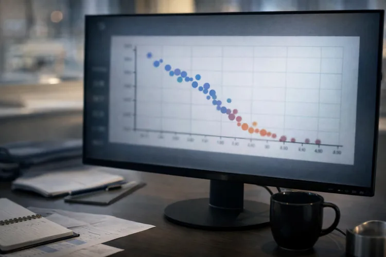
The main artifact you want is a privacy–utility curve. This lets you discuss trade‑offs quantitatively with both ML peers and clinical stakeholders.

import matplotlib.pyplot as plt

def run_sweep(
    clip_norms=(0.5, 1.0, 2.0),
    noise_multipliers=(0.7, 1.0, 1.3, 1.7),
    batch_size=64,
    epochs=15,
    lr=8e-4,
):
    results = []
    N = len(train_ds)
    delta = 1.0 / (10 * N)

    for C in clip_norms:
        for sigma in noise_multipliers:
            print(f"\n--- Sweep: C={C}, sigma={sigma} ---")

            model, pe, _ = train_dp(
                batch_size=batch_size,
                lr=lr,
                epochs=epochs,
                noise_multiplier=sigma,
                max_grad_norm=C,
                delta=delta,
            )

            val_loader = DataLoader(val_ds, batch_size=batch_size, shuffle=False)
            val_auc, val_acc = evaluate_auc_acc(model, val_loader)
            eps = pe.get_epsilon(delta)

            results. append(
                {
                    "epsilon": float(eps),
                    "delta": float(delta),
                    "val_auc": float(val_auc),
                    "val_acc": float(val_acc),
                    "C": float(C),
                    "sigma": float(sigma),
                }
            )

    return results

results = run_sweep()

epsilons = [r["epsilon"] for r in results]
aucs = [r["val_auc"] for r in results]

plt.figure()
plt.scatter(epsilons, aucs)
plt.xlabel("Privacy loss epsilon (smaller = stronger privacy)")
plt.ylabel("Validation AUROC")
plt.title("Privacy–Utility Trade-off: AUROC vs epsilon")
plt.show()

When you look at the scatter plot, you are looking for a region where utility is clinically acceptable, and privacy loss is as small as you can make it. On small datasets, you may find the curve is steep, which is itself an important finding.

If the DP curve never reaches an acceptable AUROC, it may not mean “DP is impossible.” It may mean you need a simpler model, better features, fewer training steps, or a redefinition of the clinical label to reduce noise.

Choosing $\delta$ and reading $\varepsilon$ responsibly

$\delta$ is often set using a heuristic like $\delta = 1/(kN)$ where $k$ might be 10 or 100. The exact choice should be aligned with organizational policy and threat modeling, but the key is to be consistent and transparent.

In reports and model documentation, always state privacy as a pair: “trained with $(\varepsilon, \delta)$‑DP.” Avoid reporting only $\varepsilon$ without $\delta$, because it hides part of the guarantee.

Also, document the assumptions. Privacy accounting depends on the sampling procedure and the DP mechanism. If you change batch size, number of epochs, or sampling mode, $\varepsilon$ changes even if $\sigma$ and $C$ stay the same.

Systems and production considerations in clinical environments

DP changes what “production readiness” means. It is not enough to have good validation metrics; you also need to manage privacy budgets, training metadata, and governance artifacts in a repeatable way.

In a typical healthcare data pipeline, training is batch‑based. Features are computed from EHR extracts in controlled environments, and models are trained on a schedule. DP should be applied inside the controlled boundary, and you should be explicit about what leaves the boundary (DP model artifacts, aggregated metrics, and documentation).

Logging becomes more important, not less. Store the final $(\varepsilon, \delta)$, the DP hyperparameters $(\sigma, C)$, the batch size, epoch count, and the evaluation protocol. In clinical work, being able to reproduce and audit a training run is as important as achieving a high AUROC.

Performance also matters. DP‑SGD requires per‑sample gradients, which can increase memory usage. This may be manageable for tabular models,s but becomes a scaling constraint for large text or image models, where you may need memory‑efficient clipping modes and careful batch sizing.

Finally, secure randomness is a governance decision. Some DP implementations support “secure” random number generation for noise and shuffling, which can reduce certain attack surfaces but can slow training. In many teams, you iterate quickly in standard mode and retrain release candidates under stricter settings.

Risk, ethics, safety, and governance: DP is necessary but not sufficient

DP mitigates a specific risk: leakage of training participation through the model. It does not guarantee fairness, it does not fix biased data collection, and it does not make a model clinically valid.

Small clinical datasets amplify representativeness problems. If a subgroup is underrepresented, DP noise can disproportionately harm performance for that subgroup because the signal is already weak. This makes subgroup evaluation and careful reporting more important, not optional.

DP also does not solve calibration. A DP model can have decent AUROC and still be miscalibrated, which is dangerous when outputs are interpreted as probabilities. In clinical settings, calibration checks, threshold selection, and human‑in‑the‑loop review are part of responsible deployment.

Be careful with debugging signals. Anything that exposes per‑record behavior, such as per‑sample gradients or detailed logs, can become a leakage vector if handled incorrectly. Treat debugging artifacts as sensitive and keep them within the same controlled environment as the raw data.

From a compliance perspective, DP can strengthen a privacy posture, but it does not replace access controls, audit logging, retention policies, and clinical governance. You should think of DP as one layer in a broader safety and security stack.

Domain‑specific scenario: private readmission risk modeling for a small clinic

Consider a clinic network with around 800 patients in a care‑management program. The team wants to predict 30‑day readmission risk so nurses can prioritize follow‑up calls after discharge.

The dataset is small and sensitive. Features may include recent admissions, comorbidity indices, medication categories, lab summaries, and utilization patterns. The label may be noisy because readmissions outside the network are missing, and the positive class is likely imbalanced.

A non‑private baseline model establishes the upper bound of what is possible with the current features. Then the team trains DP models across a small sweep of $(\sigma, C)$ values and plots validation AUROC versus $\varepsilon$.

They choose the smallest $\varepsilon$ that still meets a workflow‑based utility requirement, such as adequate recall in the top risk decile. They then validate on a held‑out test set once, document the final $(\varepsilon, \delta)$, and package the model with clear caveats about intended use.

In practice, they deploy the score as decision support, not automation. Clinicians see the score alongside context, and they can override it. This is where the interdisciplinary aspect matters: the privacy guarantee supports safer model sharing and use, but clinical safety still depends on workflow design, monitoring, and human judgment.

Skills mapping and a learning path

This topic builds a valuable intersection of skills. You deepen PyTorch competence by writing clean training loops, stable evaluation code, and reproducible experiments on small datasets.

You also build privacy engineering intuition. Instead of treating privacy as an afterthought, you learn to reason about $(\varepsilon, \delta)$, the effect of sampling rate $q$, and how clipping and noise shape both privacy and convergence.

On the systems side, you practice production behaviors that matter in regulated domains. Logging DP metadata, maintaining audit trails, controlling training artifacts, and communicating limitations are part of real‑world clinical ML.

A strong next step is to extend this example with calibration metrics and a clinical operating point analysis. After that, try the same DP sweep on a public clinical‑style dataset or a synthetic EHR table, focusing on missingness handling and class imbalance.

If you want a structured path that builds these skills end‑to‑end (Python, ML, evaluation discipline, and production habits), explore Code Labs Academy’s Data Science & AI Bootcamp and map the curriculum to privacy‑aware healthcare ML workflows:
Explore the Data Science & AI Bootcamp

Conclusion

Differential privacy is one of the few tools that lets you quantify privacy risk in model training on sensitive clinical data. It turns privacy from a vague statement into parameters you can measure and document.

DP‑SGD enforces privacy through per‑sample gradient clipping and Gaussian noise, controlled primarily by $C$ and $\sigma$. The resulting privacy loss can be tracked as $\varepsilon$ for a chosen $\delta$, and it grows as training takes more steps.

On small clinical datasets, privacy budgets can be consumed quickly, so disciplined tuning and privacy–utility plots are critical. The most defensible workflow is to sweep DP settings, plot AUROC versus $\varepsilon$, and select a configuration that meets clinical utility thresholds with the strongest privacy you can afford.

DP is not a substitute for clinical validation, fairness evaluation, calibration checks, or governance. It is a powerful complement that supports safer collaboration and deployment when used with the rest of the clinical ML safety stack.